DYI Rain Prediction Using Arduino, Python and Keras

First a few words about this project the motivation, the technologies involved and the end product that we’re going to build.

So the big aim here is obviously to predict the rain in the future (we’ll try 6 hours). The prediction will be a yes or no (boolean in programming terms). I’ve searched from tutorials on this matter and i haven’t found one that is complete in every way. So mine will take this to a whole new approach and get into every aspect of it. For that we’re going to:

– build the weather station our selves. The station should be completely off grid with a solar panel, and a extremely low power mode (a few dozens microamps hour)

– program the station so it gather data and transmits it every ten minutes to a base station

– collect the data on the base station and store it (in a database)

– using neural networks (Keras library) and other python libraries like pandas filter, clean and preprocess the data, then feed it to a neural network to train a “model” for predicting that it shall or not rain

– finally predict whether or not it will rain on the next 6 hours and notify users via email

I’ve personally used this weather station to collect data (you can download the data in the next steps if you wish). With only about 600 days of weather data the system can make a prediction if it will rain or not in the next 6 hours with an accuracy of around 80% depending on the parameters which is not that bad.

This tutorial we’ll take you through all the necessary steps to predict rainfall from scratch. We’ll make an end product that does a practical job, without using external weather or machine learning API-s. We’ll learn along the way how to build a practical weather station (low power and off the grid) that really collects data over long periods of time without maintenance. After that you’ll learn how to program it using Arduino IDE. How to collect data into a database on a base station (server). And how to process the data (Pandas) and apply neural networks (Keras) and then predict the rainfall.

Step 1: Parts and Tools for Building the Station

Tools:
1. USB to serial FTDI adapter FT232RL to program the Arduino pro mini

2. Arduino IDE

3. Drill

4. Fine blade saw

5. Screwdrivers

6. Soldering iron

7. Wire cutter

Skills:

1. Soldering, check this tutorial

2. Basic arduino programming

3. Linux service configuration, package installation

4. Some programming skills

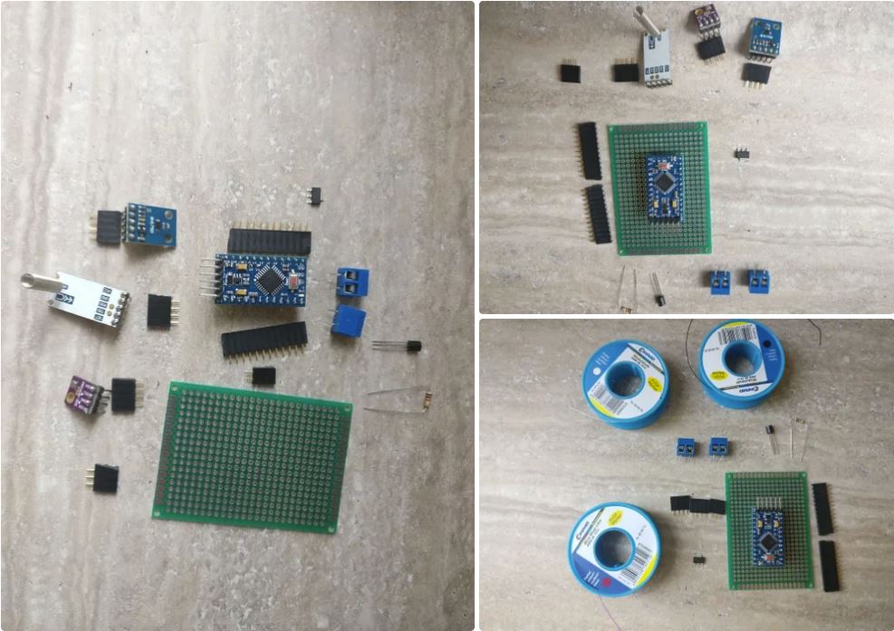
Step 2: Building the Weather Station

The weather station is composed from the following sets of components:

1. the box with the solar panel glued to it

2. the PCB with the electronics inside

3. the battery holder also inside

4. the BME280 and light and rain sensors on the outside

1. The box needs 4 holes, one for the solar panel wires, other three for the sensors that will be placed on the outside. First drill the wholes, they should be large enough for the male-female wires to stick out and go to the sensors. After the wholes are drilled, glue the panel to one side of the box and get it’s wires through a hole inside

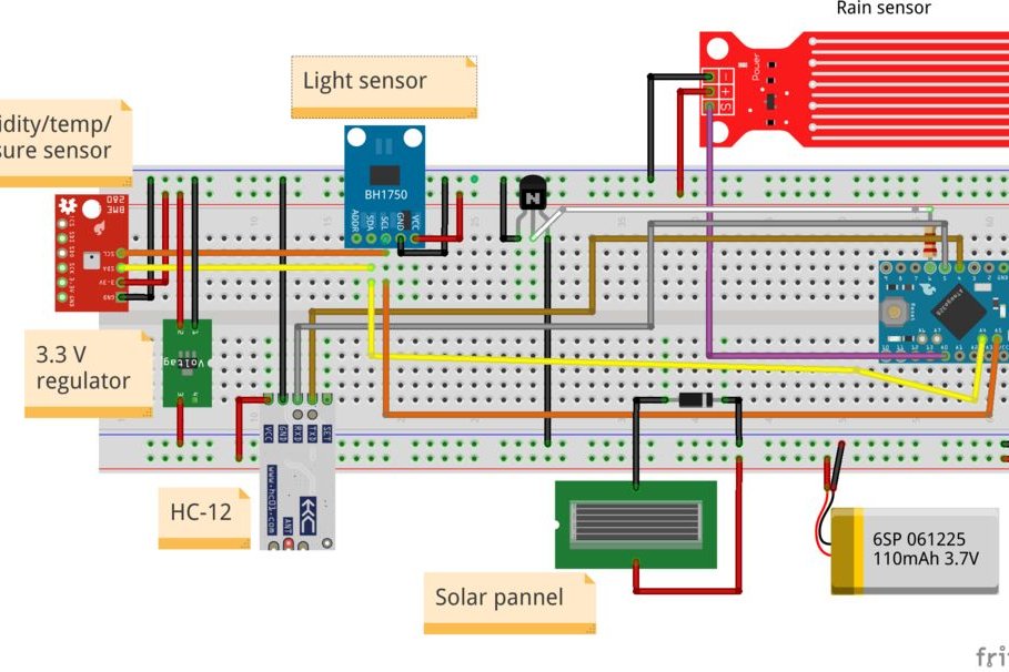
2. The PCB will hold the arduino, HC-12, 3.3V regulator, diode, transistor, resistor and two KF301-2P

– first solder the two female PCB connectors on the PCB for the arduino, solder the male pcb connectors to the arduino and place the arduino on the PCB

– the arduino led should be removed or at least one of it’s pin. this is very important because the led will draw a large amount of power. Be careful not to damage other components

– solder the transistor, resistor, and 3.3V regulator

– solder the two KF301-2P. One will be for the solar panel, the other for the battery holder

– solder three female PCB connectors: for the light sensor, BME280 and rain sensor

– solder small wires to connect all the PCB components (check the pictures and the fritzing schamatic)

3. place 3 charged AAA NiMH batteries inside the holder and place it inside the box, connecting the wires into the KF301-2P connector

4. connect the BME280 and light sensors from outside the box to their corresponding male connectors

For the rain sensor, solder three wires (Gnd, Vcc, signal) to it, and to the other side solder male pins that will go inside the box to its corresponding male connectors

The final thing it would be to place the station to it’s final position. I’ve chose a position that is sheltered from the rain and snow. I’ve chosen longer wires for the rain sensor and placed it separately in the rain on a steady support. For the main box i’ve chosen a special kind of tape with adhesive (check the pictures) but anything that holds the box will do.

Step 3: Arduino Code

The role of the weather station is to transmit to a base station every 10 minutes data about it’s sensors.

First let’s describe what the weather station program does:
1. read sensors data (humidity, temperature, pressure, rain, light, voltage)

2. transmits the encoded data through a second software serial line.

The encoded data looks like this:

The statement from above will mean that: humidity from station “1” is 78 percent, temperature from station 1 is 12 degrees, pressure is 1022 bars, light level 500 lux, rain 0, and voltage 4010 millivolts

3. power off the auxiliary components: sensors and communication device

4. puts the arduino in sleep mode for 10 minutes (this will make it consume less 50 microamps)

5. turn on the components and repeat steps 1 – 4

One little extra tweak here, if the voltage level is above 4.2 V the arduino will use the normal sleep function “delay(milliseconds)”. This will greatly increase the power consumption and decreasing the voltage rapidly. This effectively prevents the solar panel from overcharging the batteries.

You can get the code from my Github repository here:

https://github.com/danionescu0/home-automation/tree/master/arduino-sketches/weatherStation

Or copy-pasting it from below, either way just remove the line with “transmitSenzorData(“V”, sensors.voltage);”

Before uploading the code, download and install the following arduino libraries:

* BH1750 library: https://github.com/claws/BH1750
* LowPower library: https://github.com/rocketscream/Low-Power

* Adafruit Sensor library: https://github.com/adafruit/Adafruit_Sensor

* Adafruit BME280 library: https://github.com/adafruit/Adafruit_Sensor

If you don’t know how to do that, check out this tutorial.

Step 4: Preparing the Base Station

The base station will consist of a linux computer (desktop, laptop or development board) with the HC-12 USB module attached. The computer must remain always on to collect data every 10 minutes from the station.

I’ve used my laptop with Ubuntu 18.

The installation steps:

1. Install anaconda. Anaconda is a python package manager and it will make it easy for us to work with the same dependencies. We’ll be able to control the python version, and each package version

If you don’t know how to install it check out this: https://www.digitalocean.com/community/tutorials/h… tutorial and follow the steps 1 – 8

2. Install mongoDb. MongoDb will be our main database for this project. It will store data about all the sensors time series. It’s schemaless and for our purpose it’s easy to use.

For installation steps check out their page: https://docs.mongodb.com/v3.4/tutorial/install-mon…

I’ve used an older version of mongoDb 3.4.6, if you follow the tutorial above you’ll get exactly that. In principle it should work with the latest version.

3. Download the project from here: https://github.com/danionescu0/home-automation . We’ll be using the weather-predict folder

4. Create and configure anaconda environment:

This will create an new anaconda environment and install the needed packages. Some of the packages are:

Keras (high level neural network layer, with this library we’ll make all our neural network predictions)

pandas (useful tool that manipulates data, we’ll use it heavily)

pymongo (python mongoDb driver)

sklearn (data mining and data analysing tools)

Configure the project

The config file is situated in the weather-predict folder and is named config.py

1. if you install mongoDb remotely or on a different port change the “host” or “port” in the

2. Now we need to attach the HC-12 USB serial adapter. Before than run:

and you should get a list of mounted devices.

Now insert the HC-12 in a USB port and run the same command again.It should be one new entry in that list, our serial adapter. Now change the adapter port in the config if necessary

Step 5: Use the Weather Station in Practice

Here we’ll discuss basic stuff about importing my test data, running some tests on it, setting up your own data, displaying some graphs and setting up an email with prediction for the next few hours.

If you like to know more about how it works check out the next step “How does it work”

Importing my already gathered data

MongoDb comes with a cli command for importing data from json:

This will import the file from sample data into “weather” database and “datapoints” collection

A warning here, if you use my gathered data, and combine it with your newly local data the accuracy might drop because of the small differences in hardware (sensors) and local weather patterns.

Gathering new data

One of the base station roles is to store incoming data from the weather station into the database for later processing. To start the process that listens to the serial port and stores in the database just run:

Generating the prediction model

I’ll presume you have imported my data or “ran the script for a few years” to gather your personialised data, so in this step we’ll process the data to create a model used to predict future rain.

* The first parameter –days_behind means how much data into the past should the script process. It’s measured in days

* –test-file-percent means how much of the data should be considered for testing purpose, this is a regular step in a machine learning algorithm

* –hour-granularity basically means how many hours into the future we’ll want the prediction

* –datapoints-behind this parameter will be discussed further into the next section

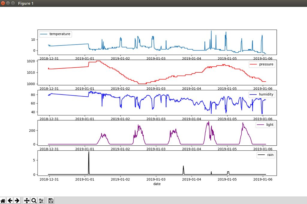
View some data charts with all the weather station sensors

Let’s say for the last 10 days:

Predict if it will rain in the next period

We’ll predict if it’s going to rain and send an notification email

Run a batch predict on the test data:

It’s important to use the same parameters as in the train script above.

For the email notification to work log in into your gmail account and Turn Allow less secure apps to ON. Be aware that this makes it easier for others to gain access to your account.

You’ll need two email addresses, a gmail address with the above option activated, and an other address where you’ll receive your notification.

If you like to receive notifications every hour, put the script into crontab

To see how all of this is possible check the next step

Step 6: How Does It Works

In this last step we’ll discuss several aspects of the architecture of this project:

1. Project overview, we’ll discuss the general architecture and technologies involved

2. Basic concepts of machine learning

3. How the data is prepared (the most important step)

4. How the actual neural network wrapper API works (Keras)

5. Future improvements

I’ll try to give some code example here but bear in mind, that it’s not 100% the code from the project. In the project it’s self the code it’s a bit more complicated with classes and a structure

1. Project overview, we’ll discuss the general architecture and technologies involved

As we talked earlier, the project has two separate parts. The weather station it’s self which only function is to collect and transmit data. And the base station where all the collection training and prediction will happen.

Advantages of the separation of the weather station and the base station:

– power requirements, if the weather station was able to process the data too, it would need substantial power, maybe large solar panels or a permanent power source

– portability, due to it’s small size the weather station can collect data from a few hundred meters away and you can easily change it’s place if needed

– scalability, you can increase the prediction accuracy by building more than one weather stations and spread them around a few hundred meters

– low cost, because it’s a cheap device you can easily build another in case one is lost or stolen

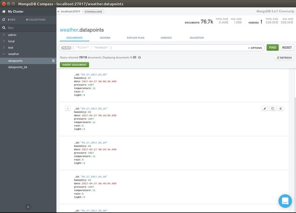
The database choice. I’ve chosen mongoDb because it’s nice features: schemaless, free and easy to use API

Every time sensor data is received the data is saved in the database, a the data entry looks something like this:

The database stores data in BSON format (similar to JSON) so it’s easy to read and easy to work with. I’ve aggregated the data under an identifier that contains the date formatted as string to the minutes, so the smallest grouping here is a minute.

The weather station (when working properly) will transmit a datapoint every 10 minutes. A datapoint is a collection of “date”, “humidity”, “pressure”, “temperature”, “rain” and “light” values.

The data processing and neural network technology choice

I’ve chosen python for the backend because many major inovations in neural networks are found in python. A growing community with a lot of Github repositories, tutorials blogs and books are here to help.

* For the data processing part i’ve used Pandas (https://pandas.pydata.org/). Pandas make working with data easy. You can load tables from CSV, Excel, python data structures and reorder them, drop columns, add columns, index by a column and many other transformations.

* For working with neural networks i’ve chosen Keras (https://keras.io/). Keras is a high level neural network wrapper over more lower level API’s like Tensorflow and one can build a multi – layer neural network with a dozen lines of code or so. This is a great advantage because we can build something useful on the great work of other people. Well this is the basic stuff of programming, build on other smaller building blocks.

2. Basic concepts of machine learning

The scope of this tutorial is not to teach machine learning, but merely to outline one of it’s possible use cases and how we can practically apply it to this use case.

Neural networks are data structures that resemble brain cells called neurons. Science discovered that a brain has special cells named neurons that communicate with other neurons by electrical impulses through “lines” called axons. If stimulated sufficiently (from many other neurons) the neurons will trigger an electric impulse further away in this “network” stimulating other neurons. This of course is a oversimplification of the process, but basically computer algorithms try to replicate this biological process.

In computer neural nets each neuron has a “trigger point” where if stimulated over that point it will propagate the stimulation forward, if not it won’t. For this each simulated neuron will have a bias, and each axon a weight. After a random initialization of these values a process called “learning” starts this means in a loop an algorithm will do this steps:

– stimulate the input neurons

– propagate the signals through the network layers until the output neurons

– read the output neurons and compare the results with the desired results

– tweak the axons weights for a better result next time

– start again until the number of loops has been reached

If you like to know more details about this process you can check out this article: https://mattmazur.com/2015/03/17/a-step-by-step-ba…. There are also numerous books and tutorials out there.

One more thing, here we’ll be using a supervised learning method. That means we’ll teach the algorithm the inputs and the outputs also, so that given a new set of inputs it can predict the output.

3. How the data is prepared (the most important step)

In many machine learning and neural network problems data preparation is a very important part and it will cover:

– get the raw data

– data cleanup: this will mean removing orphan values, aberrations or other anomalies

– data grouping: taking many datapoints and transforming into an aggregated datapoint

– data enhancing: adding other aspects of the data derived from own data, or from external sources

– splitting the data in train and test data

– split each of the train and test data into inputs and outputs. Typically a problem will have many inputs and a few outputs

– rescale the data so it’s between 0 and 1 (this will help the network removing high/low value biases)

Getting the raw data

In our case getting data for mongoDb in python is really easy. Given our datapoints collection just this lines of code will do

Data cleanup

The empty values in the dataframe are dropped

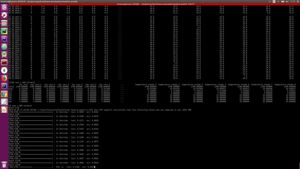
Data grouping & data enhancing

This is a very important step, the many small datapoins will be grouped into intervals of 6 hours. For each group several metrics will be calculated on each of the sensors (humidity, rain, temperature, light, pressure)

– min value

– max value

– mean

– 70, 90, 30, 10 percentiles

– nr of times there has been a rise in a sensor

– nr of times there has been a fall in a sensor

– nr of times there has been steady values in a sensor

All of these things will give the network information for a datapoint, so for each of the 6 hours intervals these things will be known.

From a dataframe that looks like this:

And the transformation will be:

After this a new column named “has_rain” will be added. This will be the output (our predicted variable). Has rain will be 0 or 1 depending if the rain average is above a threshold (0.1). With pandas it’s as simple as:

Data cleanup (again)

– we’ll drop the date column because it’s no use to us, and also remove datapoints where the minimum temperature is below 0 because our weather station it doesn’t have a snow sensor, so we won’t be able to measure if it snowed

Data enhancing

Because data in the past might influence our prediction of the rain, we need for each of the dataframe rows to add columns reference to the past rows. This is because each of the row will serve as a training point, and if we want the prediction of the rain to take into account previous datapoints that’s exactly what we should do add more columns ex:

So you see that for every sensor let’s say temperature the following rows will be added: “temperature_1” , “temperature_2” .. meaning temperature on the previous datapoint, temperature on the previous two datapoints etc. I’ve experimented with this and i found that a optimum number for our 6 hour groupings in 8. That means 8 datapoints in the past (48 hours). So our network learned the best from datapoins spanning 48 hours in the past.

Data cleanup (again)

As you see, the first few columns has “nan” values because there is nothing in front of them so they should be removed because they are incomplete.

Also data about current datapoint should be dropped, the only exception is “has_rain”. the idea is that the system should be able to predict “has_rain” without knowing anything but previous data.

Splitting the data in train and test data

This is very easy due to Sklearn package:

This will split the data randomly into two different sets

Split each of the train and test data into inputs and outputs

Presuming that our “has_rain” interest column is located first

Rescale the data so it’s between 0 and 1

Again fairly easy because of sklearn

4. How the actual neural network wrapper API works (Keras)

Building a multi layer neural network with keras is very easy:

So what does this code mean? Here we’re building a sequential model , that means sequentially all the layers will be evaluated.

a) we declare the input layer (Dense), here all the inputs from our dataset will be initializedm so the “input_dim” parameter must be equal to the row length

b) a Dropout layer is added. To understand the Dropout first we must understand what “overfitting” means: it’s a state in which the network has learned too much particularities for a specific dataset and will perform badly when confronted to a new dataset. The dropout layer will disconnect randomly neurons at each iteration so the network won’t overfit.

c) another layer of Dense is added

d) another Dropout

e) the last layer is added with one output dimension (it will predict only yes/no)

f) the model is “fitted” that means the learning process will begin, and the model will learn

Other parameters here:

– activation functions (sigmoid, relu). This are functions that dictate when the neuron will transmit it’s impulse further in the network. There are many, but sigmoid and relu are the most common. Check out this link for more details: https://towardsdatascience.com/activation-function…

– kernel_initializer function (uniform). This means that all the weights are initialized with random uniform values

– loss function (mean_absolute_error). This function measures the error comparing the network predicted result versus the ground truth. There are many alternatives: https://keras.io/losses/

– metrics function (accuracy). It measures the performance of the model

– optimiser functions (rmsprop). It optimizes how the model learn through backpropagation.

– batch_size. Number of datapoints to take once by Keras before applying optimizer function

– epochs: how many times the process it’s started from 0 (to learn better)

There is no best configuration for any network or dataset, all these parameters can an should be tuned for optimal performance and will make a big difference in prediction success.

5. Future improvements

Let’s start from the weather station, i can see a lot of improving work to be done here:

– add a wind speed / direction sensor. This could be a very important sensor that i’m missing in my model

– experiment with UV rays, gas and particle sensors

– add at least two stations in the zone for better data (make some better averages)

– collect a few more years of data, i’ve experimented with just a year and a half

Some processing improvements:

– try to incorporate data from other sources into the model. You can start to import wind speed data and combine with the local station data for a better model. This website offers historical data: https://www.wunderground.com/history/

– optimize the Keras model better by adjusting: layers, nr of neurons in layers, dropout percents, metrics functions, optimiser functions, loss functions, batch size, learning epochs

– try other model architectures, for example i’ve experimented with LSTM (long short term memory) but it gived slightly poorer results)

To try different parameters on the learning model you can use

This will search through different “batch_size”, “epoch”, “optimizer” and “dropout” values, evaluate all and print out the best combination for your data.

If you have some feedback on my work please share it, thanks for staying till the end of the tutorial!